In my previous article, Demystifying Anti-Money Laundering, I explored the different activities involved in AML and what they demand from data infrastructure. One of the things that stood out was just how different those demands can be, even within a single use case like transaction monitoring.

That got me thinking about how we evaluate the infrastructure supporting these workloads.

Most data infrastructure benchmarks are designed around a particular set of operations, whether that’s ingest throughput, query performance, or processing a fixed dataset. They’re useful for understanding individual capabilities, but they don’t tell us how those capabilities behave together when executing a real workload.

For AML, that means handling new transactions, maintaining historical context, evaluating patterns of financial activity, and making the results available for further analysis. I wanted a way to reproduce that work, run it against different data architectures in a lakehouse deployment, and measure how the complete system behaves.

So, I extended Lakebench, the tool I built to deploy, score and compare data infrastructure on Kubernetes, to introduce an AML transaction monitoring workload. This article walks through the design, the decisions behind the implementation, and the output.

What Are We Actually Trying to Measure?

IBM’s AMLSim and the datasets IBM released with a NeurIPS 2023 paper are built for testing detection models. There are infrastructure benchmarks with a financial or lakehouse angle too: LDBC FinBench measures graph databases on fraud and risk queries, and Microsoft’s LST-Bench measures how Iceberg, Delta and Hudi tables perform as they change. None of them shows what happens to the infrastructure underneath transaction monitoring, with alerts that can be checked against what was planted.

The first challenge was deciding which parts of transaction monitoring needed to be represented in the benchmark. AML involves everything from customer onboarding and sanctions screening to investigations and regulatory reporting, but trying to reproduce all of that would make for a rather unwieldy experiment. I focused on the data processing behind transaction monitoring.

Transactions don’t exist in isolation. A payment might be perfectly ordinary until you consider the accounts involved, their relationships, and the activity that preceded it. Detecting suspicious behaviour often requires examining sequences of transactions, aggregating activity over time, or following money as it moves between counterparties.

History matters too. New transactions are evaluated against existing activity, so the data being maintained and read grows over time. Lakebench can run the pipeline both ways: batch, over a fixed five-year history, and continuous, with payments arriving in micro-batches and the history growing as it runs.

Old payments are also read again. When a sanctions list changes, banks rescreen past payments against the new list. Lakebench does this in batch runs, and the generator plants parties that were only paid before they were listed, so only the rescreen can find them. Full rule-change replay (changing a rule and rerunning it over history) is out of scope.

Finally, speed means little if detection misses what it was meant to find, so the benchmark has to check its own results.

Building the AML Workload

Modelling financial activity

I built a synthetic payment history based on ISO 20022 pacs.008 credit transfers, the message banks use to send customer payments to each other.

What we modelled	What we implemented	Why it matters
Financial population	Parties, accounts, counterparties and payment relationships	Detection needs relationships, not isolated rows
Historical activity	Five years of transactions in a batch. Continuous starts with two years and keeps adding two-year periods of the same bank	Gives detection historical context and creates accumulated state
Payment behaviour	Scheduled payments, activity bursts and temporal variation	Avoids unrealistically uniform transaction patterns
Suspicious activity	Planted typologies (recognised money-laundering patterns) such as structuring, layering (moving money through chains of accounts to obscure its origin) and round-tripping (money that returns to where it started)	Creates known patterns that detection rules can be scored against

At scale factor 1, the generator produces about 26.7 million payments over five years, from around 111,000 parties (the people and organisations behind the accounts). Scale sets the size of the bank, so scale 100 is a bank 100 times larger over the same five years.

The generator plants 17 types of activity: 15 behavioural typologies, plus hits against sanctions lists and lists of politically exposed persons (PEPs). Nine detection rules cover seven of the typologies and both screening types. The planted activity doesn’t try to reproduce the statistics of real criminal behaviour.

Example: structuring

Structuring means splitting transactions into smaller amounts to stay under reporting or detection thresholds. Lakebench models it as groups of related payments clustered just below a configurable threshold, which defaults to US$10,000 for US-dollar payments, borrowed from the US cash reporting threshold.

	What happens
Financial activity	A group of senders pays one beneficiary over up to three weeks. Some of those payments sit just under US$10,000; the rest are ordinary amounts.
Detection logic	The structuring rule raises an alert when 3 or more payments between $9,000 and $10,000 arrive within 24 hours, either from one sender or into one beneficiary from 3 or more senders.
Infrastructure work	Filter payments into the band, group them by sender per day and by beneficiary over a sliding 24-hour window, count distinct senders, and attach the payments that form each alert’s evidence.

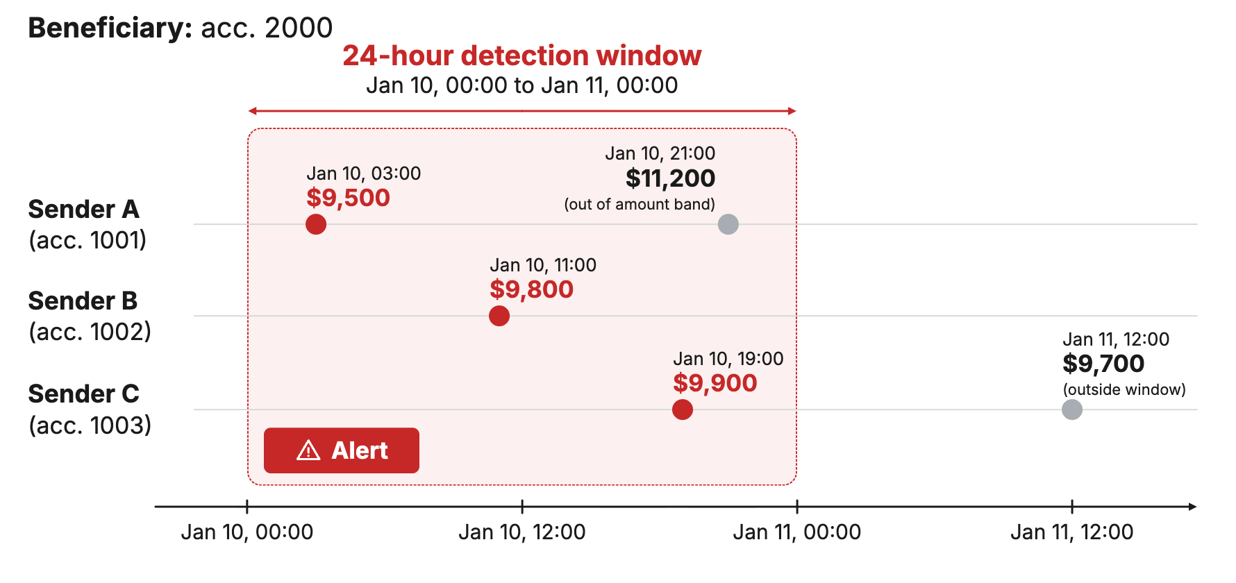
Image 1: Structuring model per account

The generator also makes detection hard on purpose. Only about 44% of structured amounts land inside the rule’s band, and campaigns run over weeks while the rule looks at 24 hours, so not every planted instance gets caught. That’s deliberate, and it’s why Lakebench reports recall (the share of planted instances the rules find) for each rule.

Turning transactions into infrastructure work

The below descriptions focus on how the pipeline maps onto a medallion processing architecture.

• Bronze registers the Parquet files into Apache Iceberg with add_files instead of reading and rewriting them. I did that to separate catalog and metadata cost from data processing cost, since a benchmark that blends the two can’t tell you which one your architecture struggles with. (Past size and file-count limits, Lakebench falls back to copying the data, and the Bronze job’s log records which path ran.)
• Silver maintains state. Each payment is appended to the double-entry ledger (a debit and a credit) and updates its account’s running balance and the sending party’s behavioural profile (running statistics that rules compare new payments against). In continuous mode, those updates are MERGEs into the entity, account and profile tables, which cover every party in the bank. The dimension MERGEs work across the whole table, so part of every batch’s cost grows with the size of the bank rather than the size of the batch.
• Gold runs the detection rules against Silver. In continuous mode, each cycle reads one Iceberg snapshot of Silver, so every rule sees the same completed payments. Each rule then reads only the period the new payments affect, plus the history it needs: two days for structuring, about six weeks for round-tripping.

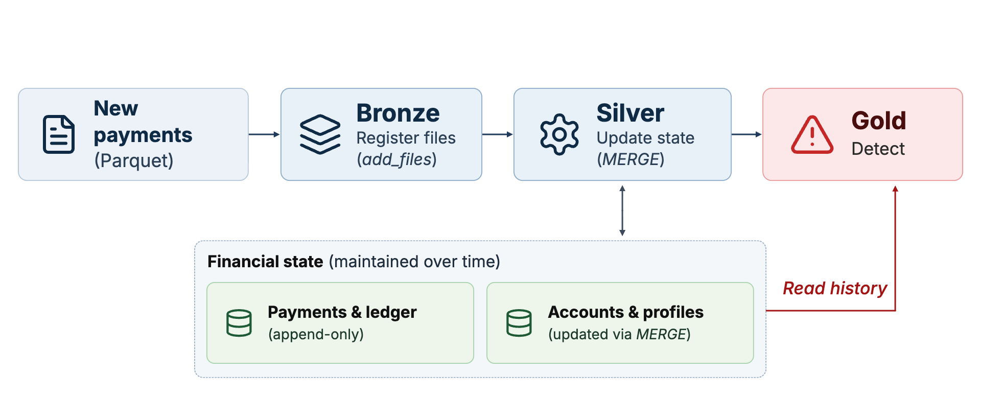
Image 2: Pipeline workflow and data architecture

At the time of writing, the AML workload doesn’t include real-time payment screening, machine-learning detection or analyst workflow.

Making the Benchmark Measurable

I wanted Lakebench to answer three questions: Did it produce the expected results? How much work did the infrastructure perform? And how did it behave as the workload progressed?

The first was the most important. Because we control the generator, we know which suspicious patterns were planted. Lakebench records them in a manifest and compares it against the alerts, so it can report recall and off-target alerts (alerts on activity that wasn’t planted for that rule) as well as timings.

In batch mode, Lakebench also fingerprints the alert set, so runs on different architectures can be confirmed to have produced the same alerts before their timings are compared.

Continuous mode is trickier, because payments keep arriving while detection runs. Lakebench scores detection only against the payments a completed detection cycle has covered, so continuous results aren’t comparable with batch.

Continuous runs also check something investigators depend on. An investigator looking at an alert weeks later needs the payments exactly as the alert saw them, which in Iceberg means time travel to the snapshot the alert read. Table maintenance expires old snapshots, so after the run Lakebench checks that each detection cycle’s snapshot still exists and times a re-read of the alert’s evidence.

AML Expirments

I ran two experiments on the same stack: a batch run at scale 100 and a one-hour continuous run at scale 20.

The experimental setup

Configuration	Batch	Continuous
Catalog	Apache Polaris 1.8.0	Same
Table format	Apache Iceberg 1.12.0	Same
Pipeline engine	Apache Spark 4.1.3	Same
Query engine	Trino 483, 4 workers	Same
Compute Infrastructure	Openshift 4.19 on Cisco C220 M5 servers with 2x Intel(R) Xeon(R) Platinum 8160 CPU @ 2.10GHz & 512GB Memory. 25GBe networking	Same
Storage	Everpure FlashBlade//S	Same
Dataset	Scale 100: 2.67 billion payments, 992 GiB in Bronze	Scale 20: 1.22 billion payments ingested in a one-hour window, about 11 years of this bank’s activity
Spark executors	28 per stage, 8 cores each (32 GB for Bronze, 64 GB for Silver and Gold)	Bronze 5 (5 cores, 10 GB), Silver 22 and Gold 15 (8 cores, 64 GB)
Table maintenance	Snapshot expiry, orphan file removal and compaction	Same, with a 30-minute snapshot retention target

Continuous experiment

The continuous run’s main finding is that Bronze kept pace with the incoming payments, Silver didn’t, and every gate still passed.

Over the hour, Bronze ingested 1.22 billion rows at 339,772 a second. That’s every row the generator wrote, so it’s the offered load, not Bronze’s capacity.

That hour delivered about 11 years of this bank’s payments, so it tests how fast the stack absorbs history, as a bank does when it backfills or reprocesses, not whether a bank this size would overwhelm it in real time.

Silver processed 1.06 billion rows at 295,619 a second, 87% of what Bronze committed, with its executors busy 86% of the time.

The pipeline passed while it fell behind

Silver takes a limited number of rows per micro-batch, so each batch took about the same time while unprocessed payments piled up behind it. Lag, which the health gates measure, rose only 38 seconds, well inside its 197-second allowance, and all five gates passed. Lakebench’s separate workload-balance check did flag that Silver wasn’t keeping up with Bronze. None of the gates measured that.

The cost of maintaining state shows up in the I/O. In the hour, Silver read 2.95 TiB from storage and wrote 399 GiB, while Bronze read 451 GiB. Silver read six and a half times what Bronze did, because its MERGEs read and rewrite existing rows in the entity, account and profile tables.

Even reading only each rule’s lookback window, Gold re-read 3.9 billion Silver rows over 21 detection cycles. Detection freshness, from a file landing to the end of the detection pass that covered it, was 867 seconds at p50 and 1,058 seconds (17.6 minutes) at p95.

The evidence check passed for all 20 detection cycles it covered.

Limits of this run:

Continuous mode runs six of the nine rules each cycle. Linked-account clusters, high-risk cross-border payments and dormant-account reactivation run in batch only, and sanctions screening checks new payments without rescreening history.

Recall is scored over the instances the last completed cycle covered (about 64% of them). It ranged from 47.1% for layering chains to 3.7% for structuring.

All three stages ran with fewer executors than Lakebench’s sizing asked for (Bronze 5 of 7, Silver 22 of 26, Gold 15 of 24), so Silver’s backlog belongs to this configuration, not to Spark, Iceberg or the storage.

Query performance as data accumulated

Three rounds of the query set ran during the continuous window. Between the first and the last, Silver’s data file count rose from 47 to 914.

Query	Round 1	Round 2	Round 3
Full scan of Silver transactions	10.9 s	28.7 s	62.2 s
Running balance for high-activity accounts	7.4 s	24.6 s	52.8 s
Top bank-to-bank corridors, last 30 days	5.6 s	4.3 s	4.3 s

The full-history queries slowed by almost six times for the full scan and seven times for the running balance. The 30-day corridor query, which only reads recent data, stayed stable. Data volume and file count were both growing, and compaction ran every 40 minutes while years of data arrived within the hour, so this run doesn’t isolate the cause.

Across the full query set, throughput fell 76% from the first round to the last, from 659.7 to 157.5 queries per hour.

Batch experiment

The batch run generated 2.67 billion payments, and Bronze, Silver and Gold took 4,593 seconds (about 76.5 minutes) from the first stage starting to the last one finishing.

Stage	Time	Read from storage	Written to storage
Datagen	498 s		992 GiB
Bronze	382 s	232 GiB	0.26 GiB
Silver	1,589 s	1,569 GiB	892 GiB
Gold	2,608 s	1,669 GiB	37 GiB
Queries	375 s	435 GiB

Bronze took the registration path. It registered the generated Parquet into Iceberg in 382 seconds, reading 232 GiB and writing only 268 MiB, where a copy would have rewritten all of it.

Silver read 1.57 TiB and wrote 892 GiB to build the payments, ledger, graph and profiles. The double-entry statements alone came to 471 GiB, larger than the 414 GiB transactions table they’re derived from.

Gold was the most expensive stage, at 57% of the pipeline time. It read 1.67 TiB from storage, about four times the 414 GiB of Silver input it was given, to produce 37 GiB of alerts.

Detection correctness

The batch run generated 72.1 million alerts, with 98.7% classified as off-target against planted instances.

The planted instances aren’t a complete label of suspicious activity. The rules evaluate every payment, and any activity that matches a rule’s conditions produces an alert, planted or not, so an off-target alert isn’t a false positive in the real-world AML sense. Those alerts still cost real compute, I/O and storage, even though 72.1 million isn’t a representative production alert rate.

Recall ranged from 99.9% for layering chains to 8.6% for structuring.

All eight benchmark queries completed. The full scan of Silver transactions took 197 seconds and the running-balance query 56 seconds, while the alert triage and investigator lookups took 4 and 6 seconds.

Limits of this run: two graph rules didn’t run at this scale. Linked-account clusters and round-tripping both hit Lakebench’s limits on graph size. The generator also produced 5.8% more data than scale 100 specifies, which Lakebench flags as outside its tolerance.

What the experiments showed

In batch, most of the work went into Gold rather than ingestion. In the continuous run, Bronze kept up while Silver built a backlog the gates didn’t catch, detection re-read billions of rows, and full-history queries slowed while a recent-window query didn’t.

Because Lakebench separates the workload from the architecture, the same experiment can be repeated with different compute and storage, and with a Polaris or Hive catalog. The AML workload itself runs on Iceberg, Spark and Trino.

The next step is making workload balance a gate, then repeating these experiments across different configurations to see which changes improve that behaviour.

The code is in Lakebench on GitHub, and the AML workload documentation covers the rules, scoring and limitations in detail. Read out if you have any workloads or ideas on how to improve the toolchain!